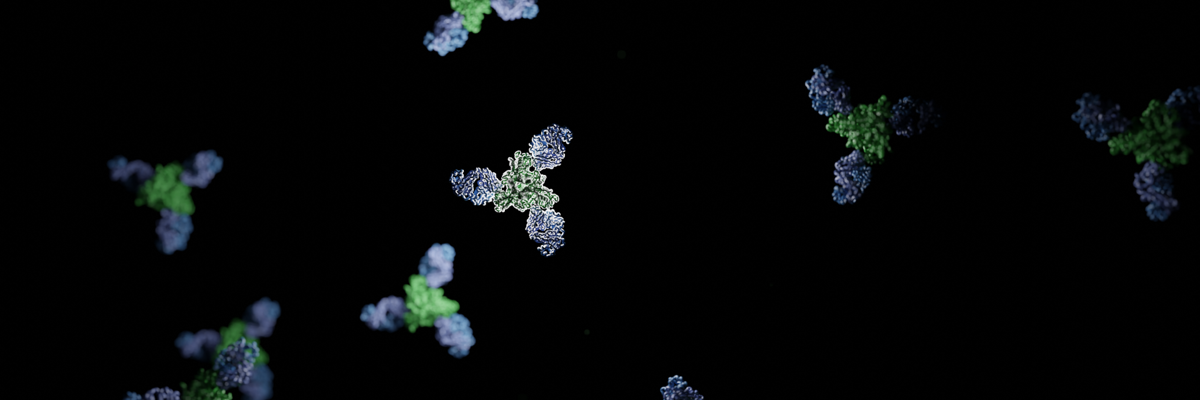
Our Manuscript is finally out! It’s been a long year since I started writing this manuscript in May 2023. As my first manuscript as the first author from my postdoctoral position, I aimed to develop tools and pipelines that would make my work on future manuscripts less tedious. This would include a resuable pipeline for generating figures for the manuscript. In this post, I will share some of the scripts I used to generate figures for the manuscript using ChimeraX.
Our paper focuses on an interesting antibody, mAb77, which was originally reported in the manuscript from 1990. mAb77 targets the measles virus (MeV) fusion glycoprotein. Since then, the single chain variable fragment (scfv) of this antibody has been the focus of another study by our collaborators from Columbia University. Further research on this mAb has shown something unusual about the mechanism of this antibody: it seems to work differently than typical glycoprotein-targeting antibodies. Specifically, this antibody seemed to block the fusion cascade rather than stabilizing the glycoprotein in the prefusion conformation.
We used single-particle cryo-EM to resolve the structure of the F-antibody complex and quickly realized that this antibody binds the prefusion conformation. However, this was confusing because the in vitro data suggested that the antibody works post-triggering (protein initiated refolding to postfusion state). We dug deeper and found out that the antibody recognizes the prefusion state but allows the glycoprotein to be triggered and start refolding. In the end (the full story can be read on Science) the antibody interaction with the glycoprotein is so strong that during refolding, it remains bound. This rigid stabilization of key domains for refolding causes the glycoprotein to split and break into pieces. In general, this was the first anti-glycoprotein antibody that showed this kind of mechanism of action. Very cool.
As I mentioned, my aim was to develop reusable tools to apply my visual style in ChimeraX for quickly rendering figures for the manuscript. ChimeraX is excellent software that offers extensive customization, is user-friendly, and supports scripting. This post will include some of the most helpful figure scripts I used for the manuscript.
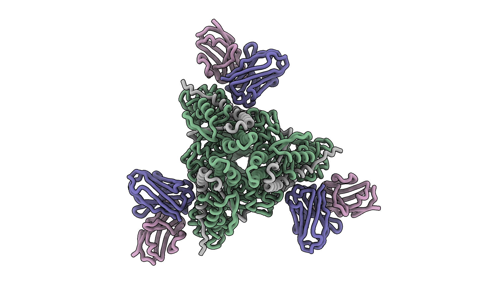
Personal preference on figure style is subjective, but I like to maintain a consistent style throughout the manuscripts. I usually start with the same visualization settings and then adjust them for each specific figure. For example, I prefer to represent secondary structures only as ribbons, which avoids the need for enforcing secondary structure definitions by refinement software or DSSP. ChimeraX allows significant modification of secondary structure visualization, so I typically use my own settings. Let’s start with loading the PDB file, setting the colors of protomers, and changing the secondary structure visualization:
# Let's open the structure of the F-Fab77 complex
open 8UT2

# set the graphics
lighting soft
hide atoms
set bgColor #ffffff00
#This setting looks not too great in the window but it is necessary for the final high resolution image
graphics silhouettes true width 5
camera ortho

# set the protein style
cartoon style protein modeHelix default arrows false xsection oval width 2 thickness 2
cartoon suppressBackboneDisplay false

show cartoon
style stick

# color chains
color #1/G,I,K #b188a7
color #1/H,J,L #6a64a5

color #1/B,D,F #72a27e
color #1/A,C,E #a7a7a7

# Save image at high resolution
save f_fab_top.png supersample 8 transparentBackground true height 2500
Those scripts can be saves as ChimeraX session files (.cxs) or can be copy-pasted into the ChimeraX command line.
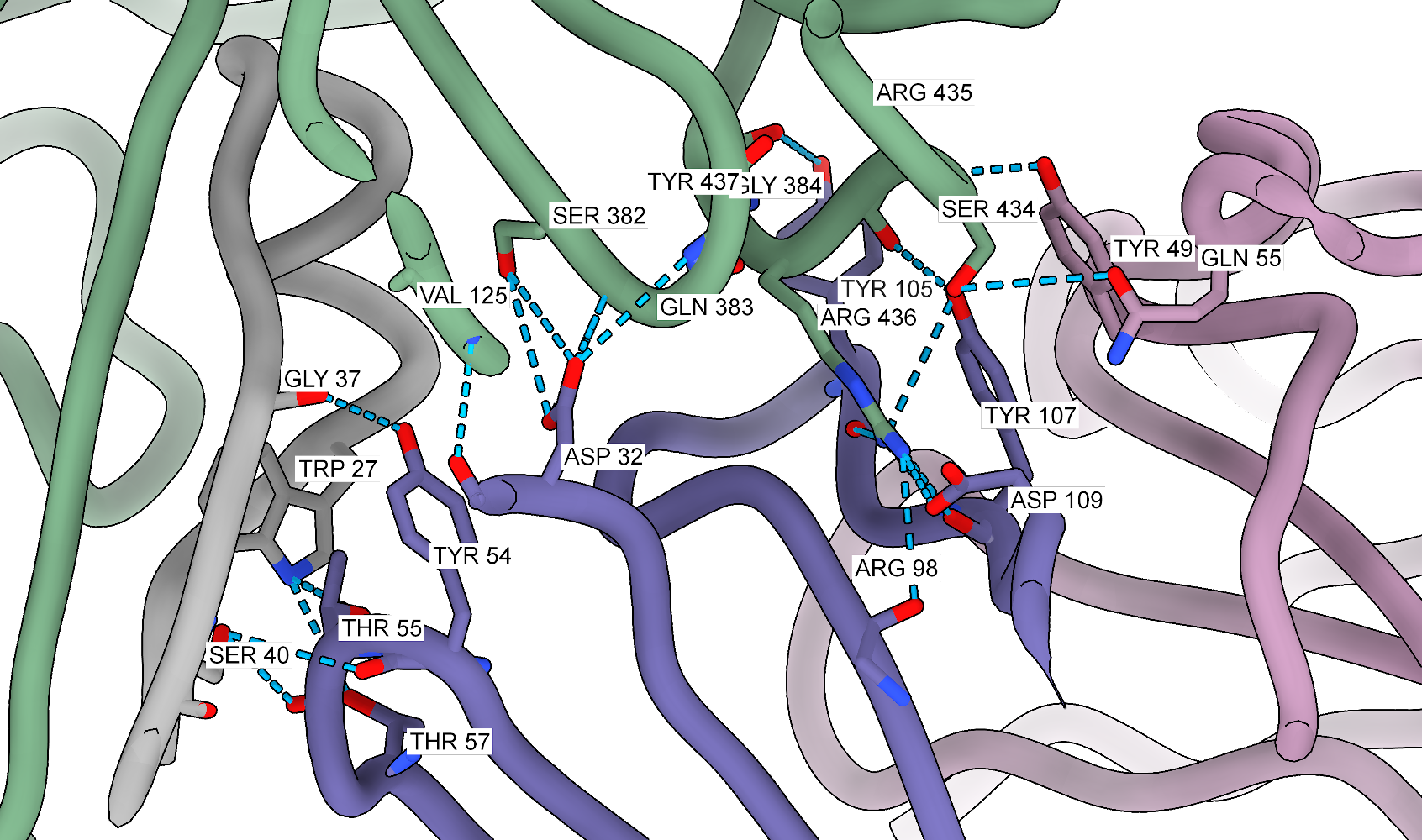
Now, we can focus on the interfaces between the antibody and Fab 77. Let’s use the previously set view matrix and change the visualization slightly to show better the interface:
view matrix camera 0.93009,-0.34248,0.13277,239.39,-0.3594,-0.92317,0.13631,202.96,0.075884,-0.1745,-0.98172,-88.695

#let's remove waters
select ::name="HOH"
delete atoms (#!1 & sel)

zoom 4
cartoon style protein modeHelix default arrows false xsection oval width 1 thickness 1

# find hydrogen bonds between F and Fab with relaxed criteria
hbonds (#1/A-F) restrict (/J,I) reveal true relax true distSlop 1.5 angleSlop 60

# color atoms by heteroatoms
color byhetero
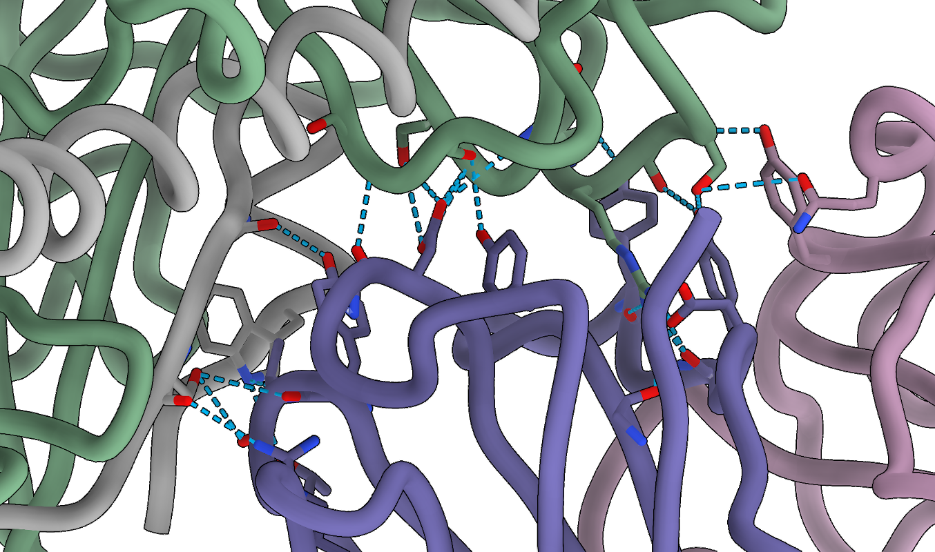
In the code above, I am using a quite permissive hydrogen bond search. For the manuscript, I used the PISA server to find the interfaces, but for a quick figure, this approach should also work. Now, we can add labels to the interacting residues. I often use this method when writing the text or preparing figures so I can see where are the residues of interest.
# hide ribbons
~ribbon
# label everything that is visible with white background
label @@display residues bgColor white
# show ribbons
show ribbons
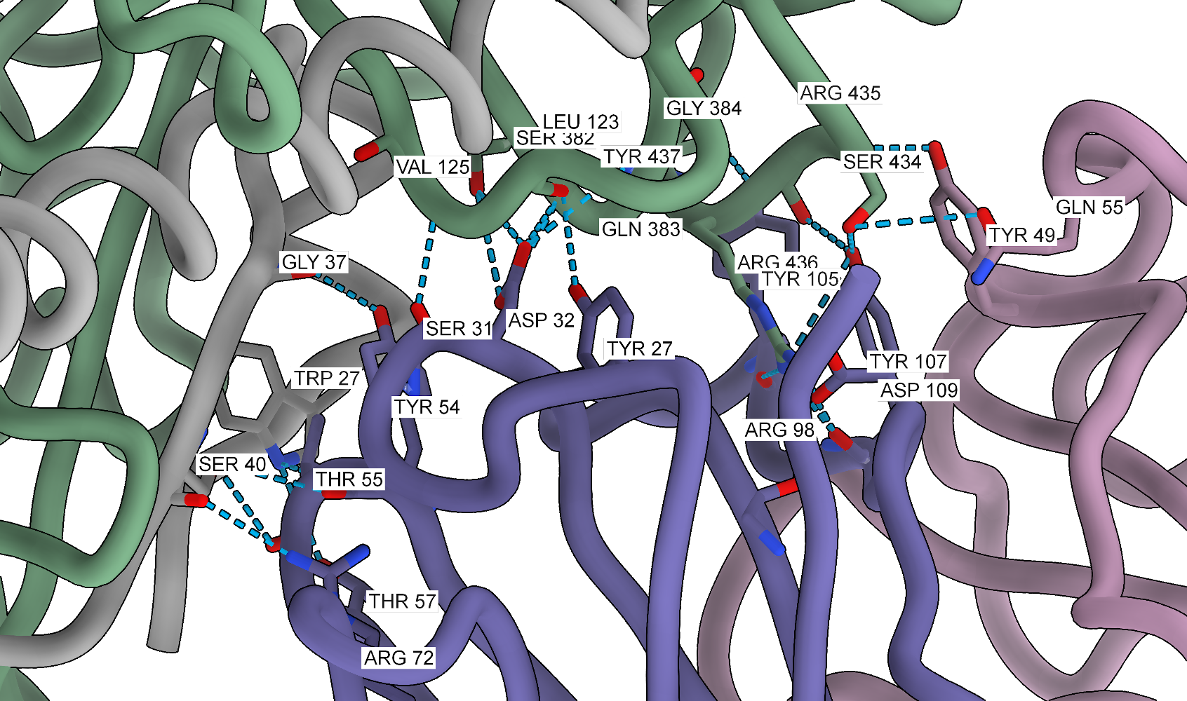
One can also experiment with clipping, although it can be more challenging to control and often requires manual adjustments for the best results. Clipping helps reduce the amount of information displayed in the figure, especially when the interface is busy. Combined with the side view tool, it can significantly improve the figure’s readability. To edit the clipping, one can use:
clip

# those values need to be adjusted on the go
clip near -10
clip far 20
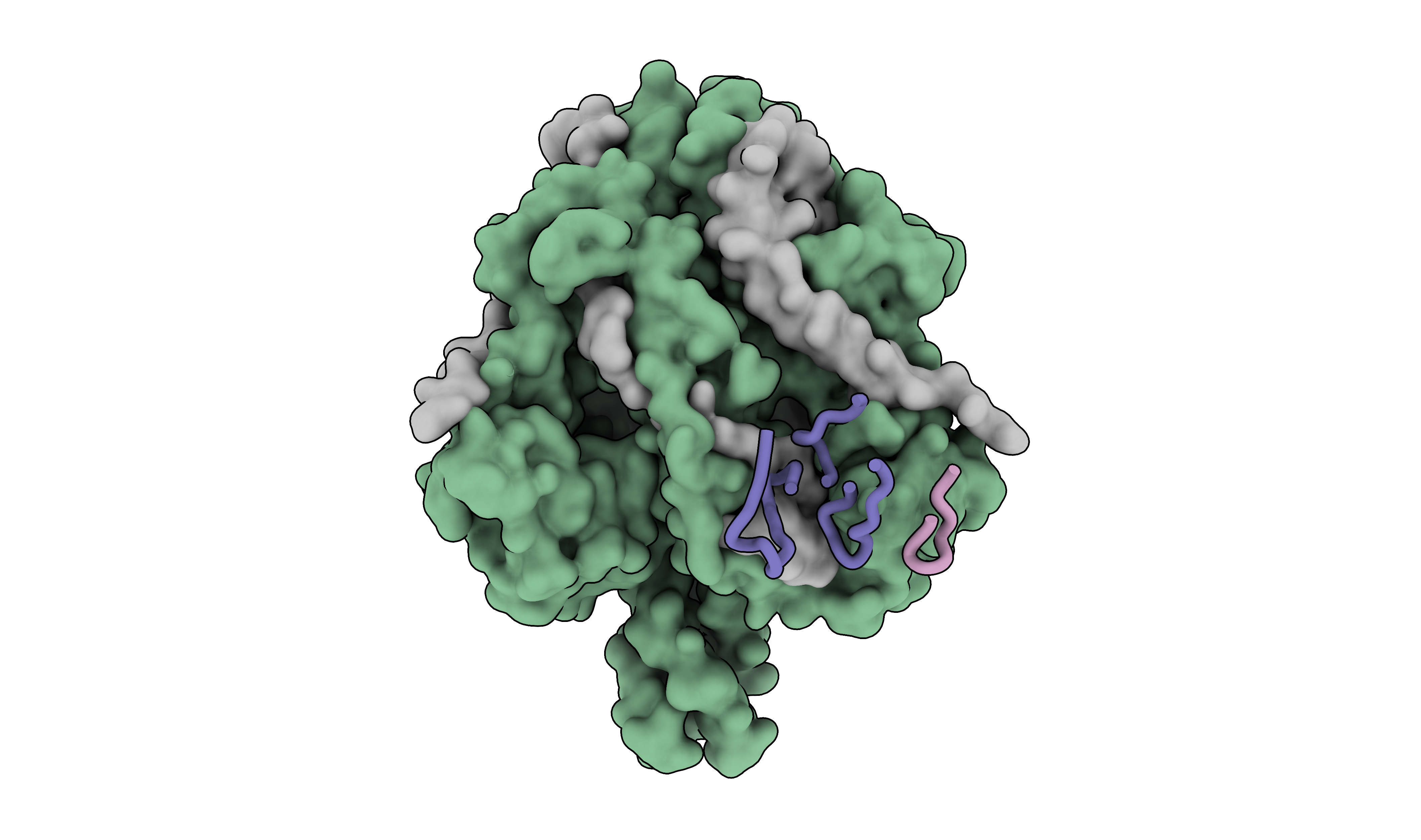
When working with antibodies, it is often useful to highlight the complementarity-determining regions (CDRs) that bind to the antigen. This can be done by selecting the residues in the CDRs and displaying them as ribbons on the surface of the antigen. I used Abysis to define the CDRs and then selected the residues in ChimeraX:
# Let's open the structure of the F-Fab77 complex
open 8UT2

# set the graphics
lighting soft
hide atoms
set bgColor #ffffff00
graphics silhouettes true width 5
camera ortho

# set the protein style
cartoon style protein modeHelix default arrows false xsection oval width 2 thickness 2
cartoon suppressBackboneDisplay false

show cartoon
style stick

# color chains
color #1/G,I,K #b188a7
color #1/H,J,L #6a64a5

color #1/B,D,F #72a27e
color #1/A,C,E #a7a7a7

# select CDRs
sel /A-F/J:99-110,26-33,53-72/I:48-56
sel ~sel; hide sel cartoon

# make the protein low resolution surface
surface #1/A-F resolution 6

view matrix camera 0.56693,0.010538,0.8237,366.31,-0.82326,0.042234,0.56609,294.56,-0.028822,-0.99905,0.032619,172.09
For the manuscript, I rendered the CDRs and protein surface in separate figures so I could adjust the transparency of the protein for easier visualization. However, for this post, I will show them together.
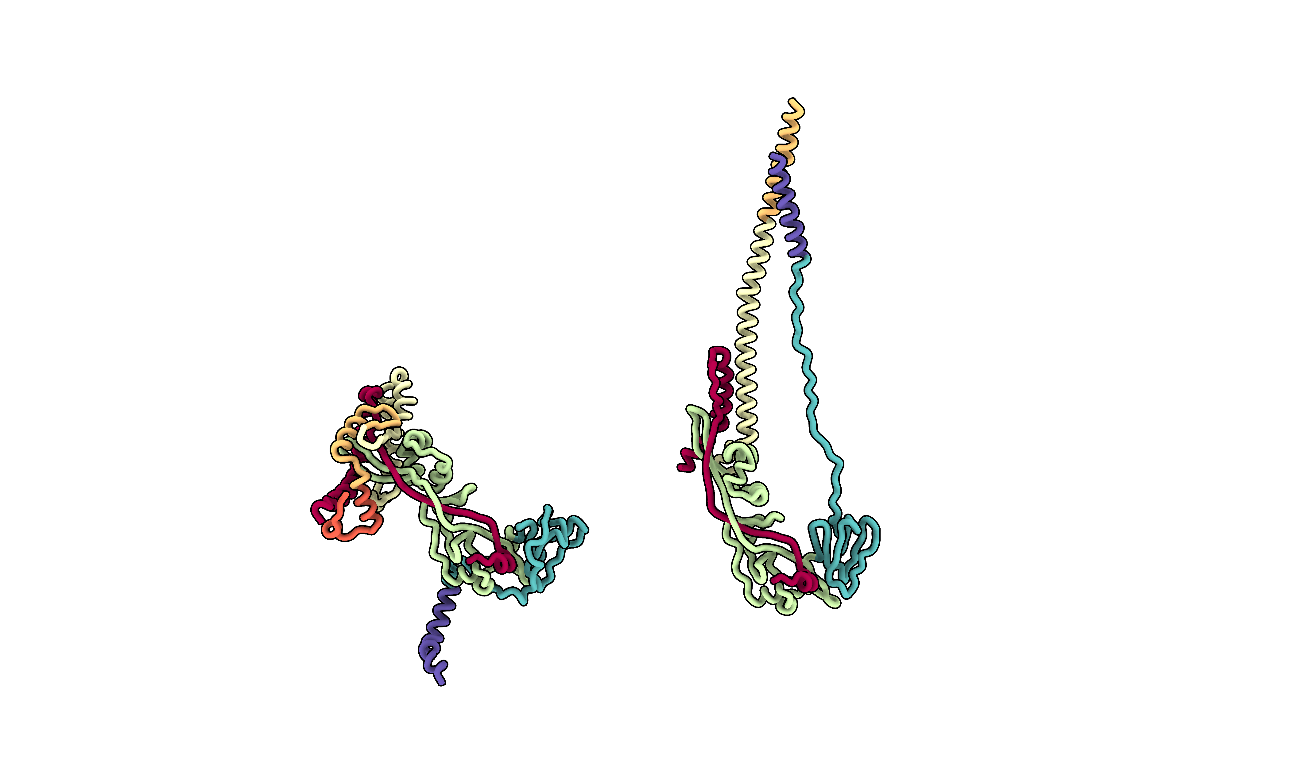
The last two figures will involve the prefusion and postfusion structures of the glycoprotein, with domain color coding for each structure or 3D sequence conservation annotation. Since the structures are not initially aligned, I will use the matchmaker command to align them first. Given the significant conformational changes between the prefusion and postfusion structures, the alignment will be based only on the region that retains a similar conformation. To generate the color scheme, I used a Python script (outside ChimeraX) to create the color scheme for the domains, which I then applied in ChimeraX.
import matplotlib.pyplot as plt
import matplotlib.colors as mcolors
from rich.console import Console

def get_hex_colors(n, colormap='coolwarm'):
    cm = plt.get_cmap(colormap)
    color_values = [x/(n-1) for x in range(n)]
    hex_colors = [mcolors.to_hex(cm(value)) for value in color_values]
    return hex_colors

console = Console()
n_colors = 7
colormap = 'Spectral'
hex_codes = get_hex_colors(n_colors, colormap)

for color in hex_codes:
    console.print(f"[{color}]{color}[/]")

domain_list_prefusion = ['#1/A', '#1/B:110-137', '#1/B:138-166', '#1/B:167-288', '#1/B:229-377', '#1/B:378-461', '#1/B:462-487']
domian_list_postfusion = ['#2/A', '#2/a:110-137', '#2/a:138-166', '#2/a:167-288', '#2/a:229-377', '#2/a:378-461', '#2/a:462-487']

for n, domain in enumerate(domain_list_prefusion):
    print(f'color {domain} {hex_codes[n]}')

for n, domain in enumerate(domian_list_postfusion):
    print(f'color {domain} {hex_codes[n]}')
This results in the ready to use ChimeraX command:
color #1/A #9e0142
color #1/B:110-137 #e95c47
color #1/B:138-166 #fdbf6f
color #1/B:167-288 #ffffbe
color #1/B:229-377 #bfe5a0
color #1/B:378-461 #54aead
color #1/B:462-487 #5e4fa2
color #2/A #9e0142
color #2/a:110-137 #e95c47
color #2/a:138-166 #fdbf6f
color #2/a:167-288 #ffffbe
color #2/a:229-377 #bfe5a0
color #2/a:378-461 #54aead
color #2/a:462-487 #5e4fa2
Here is the ChimeraX script to generate the figure:
open 8UUP
open 8UTF

lighting soft
hide atoms
show cartoon
set bgColor #ffffff00
graphics silhouettes true width 5
camera ortho
lighting model #1,2  depthCue false

cartoon style protein modeHelix default arrows false xsection oval width 2 thickness 2

mmaker #1/B to #2/a
hide #1/C-F cartoons
hide #2/B,b,C,c cartoons

color #1/A #9e0142
color #1/B:110-137 #e95c47
color #1/B:138-166 #fdbf6f
color #1/B:167-288 #ffffbe
color #1/B:229-377 #bfe5a0
color #1/B:378-461 #54aead
color #1/B:462-487 #5e4fa2
color #2/A #9e0142
color #2/a:110-137 #e95c47
color #2/a:138-166 #fdbf6f
color #2/a:167-288 #ffffbe
color #2/a:229-377 #bfe5a0
color #2/a:378-461 #54aead
color #2/a:462-487 #5e4fa2

view matrix camera -0.97265,0.021782,-0.23124,154.35,0.23179,0.027597,-0.97237,83.042,-0.014799,-0.99938,-0.031891,174.54

# Move postfusion structure
move x 100 1 models #2

# Save image at high resolution
save f_domains.png supersample 8 transparentBackground true height 2500
One might be also interested in the morph between the two states. Fortunately, ChimeraX has a built-in morphing tool that can be used to generate a movie or a series of images. Here is the script to generate the morph:
# let's redo the alignment
open 8UUP
open 8UTF

lighting soft
hide atoms
show cartoon
set bgColor #ffffff00
graphics silhouettes true width 5
camera ortho
lighting model #1,2  depthCue false

cartoon style protein modeHelix default arrows false xsection oval width 2 thickness 2

mmaker #1/B to #2/a
hide #1/C-F cartoons
hide #2/B,b,C,c cartoons

color #1/A #9e0142
color #1/B:110-137 #e95c47
color #1/B:138-166 #fdbf6f
color #1/B:167-288 #ffffbe
color #1/B:229-377 #bfe5a0
color #1/B:378-461 #54aead
color #1/B:462-487 #5e4fa2
color #2/A #9e0142
color #2/a:110-137 #e95c47
color #2/a:138-166 #fdbf6f
color #2/a:167-288 #ffffbe
color #2/a:229-377 #bfe5a0
color #2/a:378-461 #54aead
color #2/a:462-487 #5e4fa2

view matrix camera -0.97265,0.021782,-0.23124,154.35,0.23179,0.027597,-0.97237,83.042,-0.014799,-0.99938,-0.031891,174.54

# Let's remove unnecessary chains
select #1/C-F
delete atoms sel

select #2/B,b,C,c
delete atoms sel

# Morph the structures
morph #1-2

# redefine secondary structure visualization
cartoon style protein modeHelix default arrows false xsection oval width 2 thickness 2

# Record movie
movie record format PNG directory /home/dzyla/Pictures/morph/ supersample 8 size 3812,2500

# Now you need to manually click the morph play button to start saving movie frames and it will take a while

# Stop recording
movie stop
To render the final movie, one can use this Python script wrapper around ffmpeg to create a video from the images:
import os
import subprocess

def create_video_from_images(input_folder, output_video, frame_rate=16, crf=23):
    """
    Create a high-quality video from a folder of PNG images while keeping the file size small.

    Parameters:
    - input_folder: The folder containing PNG images.
    - output_video: The name of the output video file.
    - frame_rate: Frame rate of the video.
    - crf: Constant Rate Factor for controlling the quality (lower means better quality).
    """
    # Ensure the input folder exists
    if not os.path.isdir(input_folder):
        raise FileNotFoundError(f"The input folder {input_folder} does not exist.")

    # Create the ffmpeg command
    command = [
        'ffmpeg',
        '-framerate', str(frame_rate),
        '-i', os.path.join(input_folder, 'chimovie_ZvoV-%05d.png'),  # Adjust the pattern as necessary[!!!!]
        '-c:v', 'libx264',
        '-crf', str(crf),
        '-pix_fmt', 'yuv420p',
        output_video
    ]

    # Run the ffmpeg command
    try:
        subprocess.run(command, check=True)
        print(f"Video successfully created: {output_video}")
    except subprocess.CalledProcessError as e:
        print(f"An error occurred while creating the video: {e}")

# Example usage
input_folder = '/home/dzyla/Pictures/morph/'
output_video = '/home/dzyla/Pictures/morph/fecto.mp4'
create_video_from_images(input_folder, output_video)
The final video can be viewed below:
The final figure maps sequence conservation onto the structure. With the new versions of ChimeraX, this process is straightforward and requires a structure file and a multiple sequence alignment (MSA) file. For this example, I calculated the MSA for all paramyxoviruses using the UniProt query: (taxonomy_id:11158) AND (reviewed:true) AND (gene:F). To visualize the conservation on the 3D structure, let’s start a new session in ChimeraX and load all the necessary files:
open 8UUP
open 8UTF

lighting soft
hide atoms
show cartoon
set bgColor #ffffff00
graphics silhouettes true width 5
camera ortho
lighting model #1,2  depthCue false


cartoon style protein modeHelix default arrows false xsection oval width 3 thickness 3

# Align the structures
mmaker #1/B to #2/a

# Hide other chains
hide #1/C-F cartoons
hide #2/B,b,C,c cartoons

# Move the postfusion structure
move x 100 1 models #2

# Load the multiple sequence alignment
open all_paramyxo_msa.fasta

# Color cartoon by sequence conservation
color byattribute r:seq_conservation #1-2 target sabc palette -1.704,#ff2600:-1,#ffc04d:2.516,#dedddaff

# Add the color key
key #ff2600:Low #ffc04d: #dedddaff:High size 0.2, 0.02 pos 0.5, 0.08 ticks true tickThickness 2 fontSize 20
2dlab text 'Sequence conservation' xpos .495 ypos .1 bold true size 20

# Set the view matrix
view matrix camera -0.94024,0.058393,-0.33545,104.71,0.33802,0.041318,-0.94023,93.462,-0.041043,-0.99744,-0.058586,167.04
zoom 0.4

# Save the image
save conservation.png supersample 8 transparentBackground true height 2500
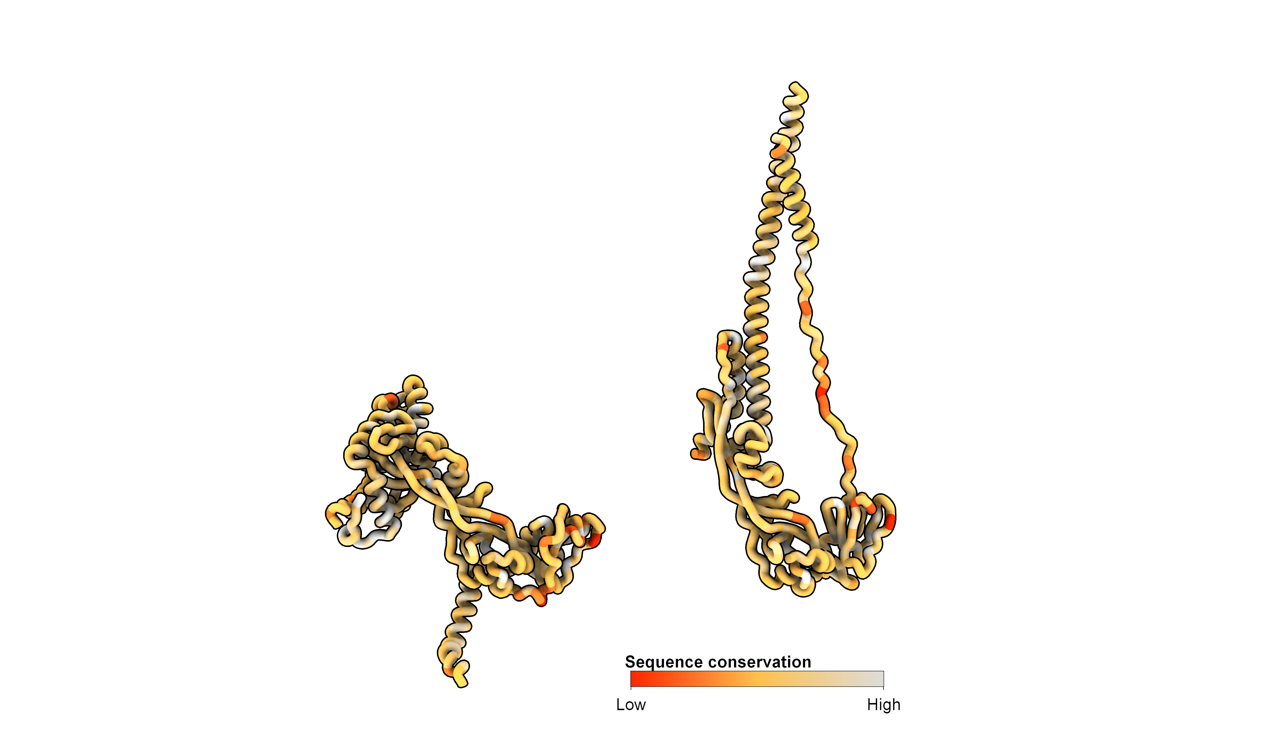
With these few scripts, I was able to generate most of the figures for the manuscript. These scripts should provide a starting point for creating publication-quality figures using ChimeraX. If you have any questions, need help with ChimeraX, or would like to see additional figure scripts, please feel free to ask in the comments. I hope you find these scripts useful and that they will assist you in your future work!